Machine learning has become increasingly popular across science, but do these algorithms actually “understand” the scientific problems they are trying to solve? In this article we explain physics-informed neural networks, which are a powerful way of incorporating physical principles into machine learning.
A machine learning revolution in science
Machine learning has caused a fundamental shift in the scientific method. Traditionally, scientific research has revolved around theory and experiment: one hand-designs a well-defined theory and then continuously refines it using experimental data and analyses it to make new predictions.
But today, with rapid advances in the field of machine learning and dramatically increasing amounts of scientific data, data-driven approaches have become increasingly popular. Here an existing theory is not required, and instead a machine learning algorithm can be used to analyse a scientific problem using data alone.
Learning to model experimental data
Let’s look at one way machine learning can be used for scientific research. Imagine we are given some experimental data points that come from some unknown physical phenomenon, e.g. the orange points in the animation below.
A common scientific task is to find a model which is able to accurately predict new experimental measurements given this data.
One popular way of doing this using machine learning is to use a neural network. Given the location of a data point as input (denoted  ), a neural network can be used to output a prediction of its value (denoted
  ), as shown in the figure below:
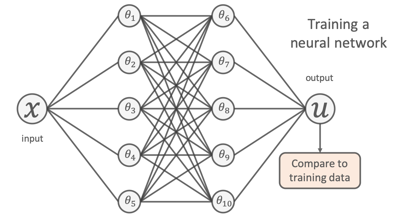
To learn a model, we try to tune the network’s free parameters (denoted by the  s in the figure above) so that the network’s predictions closely match the available experimental data. This is usually done by minimising the mean-squared-error between its predictions and the training points;
![\[\mathrm{min}~&\frac{1}{N} \sum^{N}_{i} (u_{\mathrm{NN}}(x_{i};\theta) - u_{\mathrm{true}}(x_i) )^2\]](https://benmoseley.blog/wp-content/ql-cache/quicklatex.com-6d5ab22a997dad99353f6f83b9e5f092_l3.png "Rendered by QuickLaTeX.com")
The result of training such a neural network using the experimental data above is shown in the animation.
The “naivety” of purely data-driven approaches
The problem is, using a purely data-driven approach like this can have significant downsides. Have a look at the actual values of the unknown physical process used to generate the experimental data in the animation above (grey line).
You can see that whilst the neural network accurately models the physical process within the vicinity of the experimental data, it fails to generalise away from this training data. By only relying on the data, one could argue it hasn’t truly “understood” the scientific problem.
The rise of scientific machine learning (SciML)
What if I told you that we already knew something about the physics of this process? Specifically, that the data points are actually measurements of the position of a damped harmonic oscillator:
This is a classic physics problem, and we know that the underlying physics can be described by the following differential equation:
![\[m\frac{d^2u}{dx^2} + \mu \frac{du}{dx} + k u = 0\]](https://benmoseley.blog/wp-content/ql-cache/quicklatex.com-afa121149580f9a55acb9d772e335041_l3.png "Rendered by QuickLaTeX.com")
Where
 is the mass of the oscillator,
  is the coefficient of friction and
  is the spring constant.
Given the limitations of “naive” machine learning approaches like the one above, researchers are now looking for ways to include this type of prior scientific knowledge into our machine learning workflows, in the blossoming field of scientific machine learning (SciML).
So, what is a physics-informed neural network?
One way to do this for our problem is to use a physics-informed neural network [1,2]. The idea is very simple: add the known differential equations directly into the loss function when training the neural network.
This is done by sampling a set of input training locations ( ) and passing them through the network. Next gradients of the network’s output with respect to its input are computed at these locations (which are typically analytically available for most neural networks, and can be easily computed using autodifferentiation). Finally, the residual of the underlying differential equation is computed using these gradients, and added as an extra term in the loss function.
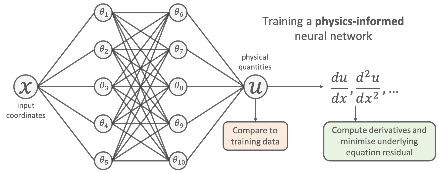
Let’s do this for the problem above. This amounts to using the following loss function to train the network:
![\begin{align*}\mathrm{min}~&\frac{1}{N} \sum^{N}_{i} (u_{\mathrm{NN}}(x_{i};\theta) - u_{\mathrm{true}}(x_i) )^2 \\+&\frac{1}{M} \sum^{M}_{j} \left( \left[ m\frac{d^2}{dx^2} + \mu \frac{d}{dx} + k \right] u_{\mathrm{NN}}(x_{j};\theta) \right)^2\end{align}](https://benmoseley.blog/wp-content/ql-cache/quicklatex.com-e464074c612008eafebb82a1faa49bde_l3.png "Rendered by QuickLaTeX.com")
We can see that the additional “physics loss” in the loss function tries to ensure that the solution learned by the network is consistent with the known physics.
And here’s the result when we train the physics-informed network:
Remarks
The physics-informed neural network is able to predict the solution far away from the experimental data points, and thus performs much better than the naive network. One could argue that this network does indeed have some concept of our prior physical principles.
The naive network is performing poorly because we are “throwing away” our existing scientific knowledge; with only the data at hand, it is like trying to understand all of the data generated by a particle collider, without having been to a physics class!
Whilst we focused on a specific physics problem here, physics-informed neural networks can be easily applied to many other types of differential equations too, and are a general-purpose tool for incorporating physics into machine learning.
Conclusion
We have seen that machine learning offers a new way of carrying out scientific research, placing an emphasis on learning from data. By incorporating existing physical principles into machine learning we are able to create more powerful models that learn from data and build upon our existing scientific knowledge.
Learn more about scientific machine learning
Want to learn more about SciML? Check out my PhD thesis, and watch our ETH Zurich Deep Learning in Scientific Computing Master’s course for a great introduction to this field!
Our own work on physics-informed neural networks
We have carried out research on physics-informed neural networks! Read the following for more:
Moseley, B., Markham, A., & Nissen-Meyer, T. (2023). Finite Basis Physics-Informed Neural Networks (FBPINNs): a scalable domain decomposition approach for solving differential equations. Advances in Computational Mathematics.
Moseley, B., Markham, A., & Nissen-Meyer, T. (2020). Solving the wave equation with physics-informed deep learning. ArXiv.
References
1. Lagaris, I. E., Likas, A., & Fotiadis, D. I. (1998). Artificial neural networks for solving ordinary and partial differential equations. IEEE Transactions on Neural Networks.
2. Raissi, M., Perdikaris, P., & Karniadakis, G. E. (2019). Physics-informed neural networks: A deep learning framework for solving forward and inverse problems involving nonlinear partial differential equations. Journal of Computational Physics.
Physics problem inspired by this blog post: https://beltoforion.de/en/harmonic_oscillator/
Hi Ben, an awesome attempt at simplifying the issue. I didn’t get the concept of simply adding the “physics” to the cost function … wouldn’t this imply that you know the answer upfront!? (in your example: the 1d wave equation” … extending on that, would it be possible to give ML access to a huge library of all known physical problems in literature (which are limited) and let ML and the “right physics” to the cost function … maybe we should have another layer of optimization that takes care of this step …
anyway fascinating subject.
Hi Amine, yes in the blog post I simply used the PINN to solve the differential equation (which can be useful by itself; i.e. the experimental data points serve as the boundary condition of the PDE). PINNs are also frequently used for inversion, where parameters in the PDE are jointly optimised alongside the network parameters (e.g. in the harmonic oscillator, one could simultaneously learn the mass/spring constant/friction coefficient too); other work has done exactly as you have described, trying to learn the actual operators in the PDE by using bi-level (sparse) optimisation: (e.g. https://arxiv.org/abs/2005.03448). There is much more to explain about PINNs that I couldn’t cover at this level, perhaps I need some more blog posts!
Some 10+ years ago ( Schmidt, M., and Lipson, H. (2009). Distilling free-form natural laws from experimental data. Science 324, 81–85. doi: 10.1126/science.1165893 ), people have tackled a somewhat complementary problem: finding the equations based on the data. Do think the two approaches can be somehow combined?
One thing is the equation, and one thing is its solution. So No, you do not know the answer upfront, you just know which test the solution needs to pass (the equation) to be accepted. What I struggle to see is the point of the of article? Does it find an analytic expression of the solution or just an opaque numerical expression that has better extrapolation properties? Eventually, what are the limits of the extrapolation? Can the approach be used for equations for which we do not know how to compute the solution?
Dear Ben,
Thanks for the amazing blogpost. Very informative. I work in computational electromagnetics and I was wondering if it is possible (or feasible) to solve an inverse problem associated with these non-linear differential equation? For example, what if we want to estimate any parameter (which is a function of space) given the physical quantity as input? For the above example of harmonic oscillator, can we estimate the coefficient of friction at different locations given the physical quantity such as speed as a function of space? Ovbiously, most inverse problems are ill-posed so we have to assume we have fewer measurements of speed (at multiple locations) and we want to estimate friction coefficient at more number of points.
Hi Amartansh,
Thanks a lot for your comment! Yes, PINNs can (and are frequently) used for inverse problems too. This is very simple conceptually – one just optimises the unknown parameters of the PDE alongside the free parameters of the network when training the network. So in the harmonic oscillator example, we could easily learn the coefficient of friction too (assuming we have enough real data points so that the inverse problem is not ill-posed, as you mention). We could also learn an unknown PDE function which varies in space too. One way would be to have another network which defines this function (and then we backpropagate through it to jointly optimise its weights and the PINN’s weights together).
This is really great and thanks for the example – helps to understand the post.
I have another question – e.g. I do not know the exact differential equation, but i know something, e.g. dimensional reasoning. i know that this problem can be described using dimensional analysis and presented as 3 or 4 non-dimensional parameters. What would be the right way to discover those combinations of dimensional parameters?
Hi Alex,
That is a really interesting idea. PINNs have also been used for learning underlying equations themselves, e.g. https://arxiv.org/abs/2005.03448. This paper uses a PINN to estimate the gradients with respect to the input coordinates of the real data points, and then does a sparse optimisation over linear combinations of these gradients to try to discover the underlying differential equation. I think doing this, and then adding a dimensional analysis constraint during the optimisation would be really interesting!
Thanks for the nice article. Just a correction that the original PINNs paper (two of them for foreward and inverse problems) was first published in 2017 in the arxiv. We didi the work in 2015-2016 time preiod and all this work is documented in the DARPA EQUiPS reports.
Thank you for nice information, Visit our web:
https://uhamka.ac.id/
Thanks for the great content! Just one question: how can we extend physics-informed machine learning models for the experimental cases where we don’t have any differential or state equations? I’m working with machine learning models for the experimental data obtained from the machinery. Do I need to have a mathematically model of the entire system in order to employ the physics-informed ML model?
Hi Ali, yes for a standard PINN, one must know the underlying differential equations so they can be used in the loss function. However, some current work tries to simultaneously train the PINN and learn the underlying differential equations at the same time, e.g. see: https://arxiv.org/abs/2005.03448
Thank for the nice comparison. However, since the considered case a dynamical system, have you compared it with Neural-ODE. Particularly, the considered example is of second-order, there is an extension of neural-ODEs for second-order systems as well (https://arxiv.org/abs/2006.07220). I would be quite interested to see this comparison than a classical NNs for an extrapolation.
Great idea Pawan. I am not an expert on neural ODEs, but to the best of my understanding, they use a neural network to describe terms in the underlying PDE, i.e., training the neural ODE would amount to learning terms in the PDE. Furthermore, a standard ODE solver is used to solve PDE during training. The difference with PINN is that no ODE solver is required, i.e. we just directly train the weights of the network. Agree, some more comparison work would be great!
what happens to the physics informed nn when you give it fewer training points? Is there a reason 9 need to be used?
Great question Philip. You can think of the PINN as a method for solving the underlying PDE. Thus, we need to provide appropriate boundary/ initial conditions so that the solution learned is unique. In PINNs, this is usually done using the training data points. For the harmonic oscillator problem above, which is a 2nd order DE, the boundary conditions I want to impose are u(0)=1 and u'(0)=0. Thus we need “enough” training points to impose these. I chose 9 randomly (and for the purpose of comparing the PINN to the NN), but I think it would be enough just to have 2 training points for this problem (as the general solution to the DE has two constants of integration).
The “naive” approach is trained for only 1000 steps, while the PINN is trained for 20,000 steps. Is the computational time per step much less in the case of the PINN? How can you compare these two models that are operating on different orders of magnitude in time?
Hi Alexander, this is a great point, the longer training times are definitely a downside for the PINN for this particular problem. I think one of the main reasons is that I had to use a smaller learning rate when training the PINN (1e-4) compared to the NN (1e-3). Using 1e-3 for the PINN made its training unstable. My hunch is that this is due to the potentially “competing” terms in the PINN loss function (one trying to match the training data, the other trying to satisfy the PDE). Related to this, the convergence of the PINN for this problem was very sensitive to the relative weighting between the two terms in the loss function. See the code for the training details: https://github.com/benmoseley/harmonic-oscillator-pinn. In terms of computational time per training step, the PINN is also slower, because the second order gradients of the network with respect to its inputs also need to be computed at each step.
I think it wouldn’t matter even if we train the “naive” approach longer because it becomes a naive extrapolation problem.
great effort
How about using reinforcement learning to train the NN? In this case it will be the agent network.
I’m currently applying time-dependent source terms in the PDEs I’m trying to predict with PINN. Does incorporating time-dependent source functions in the PDE I’m trying to predict require special considerations (higher number of epochs? smaller learning rate?… etc.)
Hi Shaikhah, I would say using a time-dependent source function does not necessarily require special considerations, because it can incorporated into the PINN loss function without any major changes to the PINN methodology. However, the convergence of PINNs is not guaranteed and depends strongly on the initial conditions and underlying PDE. So you may well need to train for longer/use a smaller learning rate etc to ensure the problem converges. Also, if the source term contains high frequencies this may be harder as PINNs often struggle to scale to higher frequency solutions, see our work here; https://arxiv.org/abs/2107.07871
Thank you for this great article and wish you the best of luck!
Good Blog! Thank you for this great article!
I wonder if the code of “Moseley, B., Markham, A., & Nissen-Meyer, T. (2020). Solving the wave equation with physics-informed deep learning. ArXiv.” can be make public? Because I did not find it on your Github home page, but found the code of another PINN article.
Hi, thanks for asking, currently the code for that paper is not available, however we do train a standard PINN (as well as a FBPINN) to solve the wave equation in our other paper you mention (paper: https://arxiv.org/abs/2107.07871) which does have code available: https://github.com/benmoseley/FBPINNs/blob/main/fbpinns/paper_main_3D.py.
Are m, mu and k supposed to be known? How does this content generalise when they are not?
Great article ! Many thanks.
Great description and demo!
I’m curious, how are you calculating your backpropagation for your custom loss function?
Hi Matthew, thankfully, I just rely on the autodifferentiation features of PyTorch; it is able to compute all of the gradients required without any extra coding effort. Here is the code: https://github.com/benmoseley/harmonic-oscillator-pinn This is because when I compute the gradients of the network with respect to its inputs using torch.autograd.grad(…, create_graph=True) PyTorch builds another computational graph which is backpropagated through when calling loss.backwards(). Hopefully that helps!
Hi Ben, first of all thank you for this very nice mechanical project.
I tried to use your example to solve the ode of the inverse pendulum.
The NN with two outputs works fine, but adding the physics loss does not help to extrapolate the equations (after more than 200.000 episodes).
You can find my code here: https://github.com/lennart2810/InvertedPendulumSDS/blob/master/PINN/InvertedPendulum/Inverse%20Pendulum%20PINN.ipynb
I apreciate any kind of advice.
Hi Lennart, super cool application of PINNs to the inverse pendulum. I replied on github via an issue on your repo 🙂
Hi Ben,
Thank you for the wonderfully simple conceptual explanation of PINNs. There is only one piece I can’t quite get my head around. That is how you derived your second term in the loss function for the physics. I would have assumed you would want to minimize the RMSE of the first and second derivatives of the spring equation with the first and second derivatives of the NN but it looks like you just put the spring equation in multiplied by the predicted output of the NN, not the gradient of the NN. So, won’t the physics equation for the spring always be zero by definition? I don’t see what is getting minimized in that second term.
I suspect I missing something obvious.
Thanks!
Scott
Hi Scott, good question, the square brackets in the physics loss denote that the derivative operators should be evaluated using the NN, rather than just applying a multiplication. So to evaluate the physics loss we must compute the gradients of the NN (dNN/dx, dNN/dx2) at the input coordinates, combine them to form the underlying equation and minimise the residual of this to train the PINN.
Hi,
First, I would like to thank you for your amazing explanation. I have a newbie question : what happens if you want to study other initial conditions (for the same equation) once your neural network is trained ? Do you have to train another neural network with the initial condition that you want, or can you use your network for any initial conditions ?
Thank you very much,
Alix
Hi Alix, it possible to add the initial condition as an extra input to the neural network so that it learns a surrogate model across different conditions. When training the PINN you would need to sample from this initial condition as well as using random input points so that it learns to generalise across this. This is potentially very useful as you would then not need to retrain the PINN for carrying out different simulations, but it is potentially harder to train the PINN too. The other option is to just retrain the PINN for each new simulation.
Hi Ben,
Very informative blog , appreciate your effort.
I am trying to use PINN for transient heat transfer problem and I need to introduce wall heat flux rate as an input. How can I create a surrogate model so that it learns for different initial conditions? . Any lead is also highly appreciated
thanks for sharing
Hi,
Thanks for sharing this blog, very informative! I’m very new into this field, and cant get my head around something about the code you provided. How exactly does the structure of the network look like in the hidden layers since nn.sequential is applied twice? I’m trying to make a PINN from scratch but have been unsuccessful so far with only ordinary dense networks.
Regards,
Bas
Hi Ben, great work!
I was looking through your code and was wondering what is the use of the 1e-4 coefficient on the physics loss computation.
Thank you and keep up the good job!
Regards,
Kit
Hi Kit,
Very good question. And I’m also very confused about the magical number (1e-4). do you have some ideas about that?
Thank you and keep up the good job.
Cheers,
Alex
Hi!
Just found this article on LinkedIn. I am looking for ways to predict weather and am working with LSTMs for now. I have read a paper published in the Royal Society about PINN and case studies with weather prediction. So, asking from a noob perspective, what would be better? LSTM or PINN or can we just use PINN while modelling through LSTM in just the loss function estimation?
I don’t understand the advantage of using a NN here because since you seem to know the model could you just have used a traditional optimization fitting method to do the fit and it would probably be quicker too. Is that right?
Wow. That is amazing. Thanks for such a great post. All we need is to merge the physics of a domain (in PDE form) with ML. Can you suggest some sources to learn about PDE?
Physics is about making model of reality not to impose on reality its limited math. So even with SciML we introduce bias of mathematical perfectionism and scientific “narrative”.
This blog is amazing. I’m curious about the hybrid FEM and PINNs. How do we integrate both like at what point Pinn’s hold and what fem will use? Like I want to solve a PDE and I want the accuracy of FEM and speed of the Neural network. At what point it should be integrated.
Hi Ben,
Firstly i would like to thank you for explaining the topic so nicely.
I have few questions regarding the initialization of the ODEs/PDEs parameter in inverse PINN.
1. What happens if the parameter values are large in magnitude (say in 100s)?
2. How to architect the NN when we have 2 or more parameters of different magnitude range (say 0.1 and 100) ?
Thank you, very good blog and very helpful
Hello,
Thank you for providing such resources about PINNS, i am working on PINNs applied to projectile motion and here i am dealing with an System ODE and i need to predict the trajectory and the paramaters of the equation! recently i found some bad convergence of model with such data so i adjust manually the loss physic with 1e-5,it improve the parameters estimation hence i can not found an explanation why such minimization of the physic loss could help to estimater the parameters however the initial physic loss=30 not considered as huge . i found your guthub code of osccilator equation with pinns and you applied a weight too for physic loss.
thank you prof i am now doing the thesis in using pinn for parapmeters estimation i am master of nuclear engineering student i am into spending some monthes with you to learn on how to better implement pinn for my case .
Hi Ben,
This is really a great read! I am a science communicator, and I am very interested in learning how you created your neat figures and animation. Could you perhaps share more details on the tools/platforms you used?
Thank you!
This is a very informative article that uses very simplified language.
Hello. I want to train a PINN but instead of differential equation, I have an Integral equation, please tell me how to do it. Like there are functions like autodifferentiation to find physics loss when we are dealing with differential equations, but how to go about in case of Integral equations.
Great insights, Ben! I appreciate how you explained the integration of physics with neural networks. It’s fascinating to see how this approach can enhance predictive modeling in complex systems. Looking forward to more in-depth discussions on its applications!
This post brilliantly breaks down the concept of physics-informed neural networks! I appreciate how you explained the integration of physics principles with deep learning. It really clarifies how they can improve modeling accuracy in complex systems. Looking forward to seeing more applications of this technology!
This post does an excellent job of breaking down the concept of physics-informed neural networks! I appreciate how you explained the integration of physical laws with machine learning, making it accessible even for those new to the topic. I’m excited to see how this approach could revolutionize problem-solving in physics and engineering!
If I already have a well-defined model of my system but want to train a Physics-Informed Neural Network (PINN) to produce outputs much faster than my current solver, would this be considered a forward or an inverse PINN problem?
Another question, do we also consider splitting our data in PINNs, training and validation sets?
This post does an excellent job of breaking down the concept of physics-informed neural networks! I appreciate how you connected deep learning with physical principles, making the topic more accessible. Looking forward to seeing more applications of PINNs in different fields!
Great post, Ben! I found the explanation of physics-informed neural networks really insightful. It’s fascinating how they can integrate physical laws with data-driven models. I’m curious about potential applications in real-world problems—do you think they could significantly improve predictive accuracy in complex systems?
This post provides an excellent overview of physics-informed neural networks! I especially appreciated how you explained their potential to bridge the gap between data-driven approaches and fundamental physics principles. Looking forward to seeing more applications of these techniques in the future!
This is a fascinating overview of physics-informed neural networks! I loved how you explained their importance in bridging the gap between data-driven approaches and traditional physics models. It’s exciting to see how these networks can enhance complex simulations. Looking forward to your future posts on this topic!
This post does a great job of explaining physics-informed neural networks (PINNs) in a clear and approachable way. I especially appreciate how it bridges the gap between deep learning and physical principles, making a complex topic easier to understand. The potential applications of PINNs across science and engineering are truly exciting, and I’m looking forward to seeing how this field continues to evolve. Thanks for sharing such an insightful overview!
Excellent explanation of physics-informed neural networks! The way you combined machine learning concepts with real-world physical constraints made the topic much easier to grasp. It’s exciting to see how PINNs can improve modeling and simulation across so many disciplines. Thanks for sharing this informative post—I’m looking forward to learning more about their practical applications and future developments.
This post does an excellent job of explaining physics-informed neural networks in a clear and engaging way. I especially appreciated how it connected physical laws with machine learning concepts, making a complex topic much easier to understand. The practical insights and real-world applications were particularly interesting. It’s exciting to see how this innovative approach could transform problem-solving in physics, engineering, and other scientific fields. Great work!