So, what is a physics-informed neural network?

Machine learning has become increasingly popular across science, but do these algorithms actually “understand” the scientific problems they are trying to solve? In this article we explain physics-informed neural networks, which are a powerful way of incorporating physical principles into machine learning.

A machine learning revolution in science

Machine learning has caused a fundamental shift in the scientific method. Traditionally, scientific research has revolved around theory and experiment: one hand-designs a well-defined theory and then continuously refines it using experimental data and analyses it to make new predictions.

But today, with rapid advances in the field of machine learning and dramatically increasing amounts of scientific data, data-driven approaches have become increasingly popular. Here an existing theory is not required, and instead a machine learning algorithm can be used to analyse a scientific problem using data alone.

Learning to model experimental data

Let’s look at one way machine learning can be used for scientific research. Imagine we are given some experimental data points that come from some unknown physical phenomenon, e.g. the orange points in the animation below.

A common scientific task is to find a model which is able to accurately predict new experimental measurements given this data.

Fig 1: example of a neural network fitting a model to some experimental data

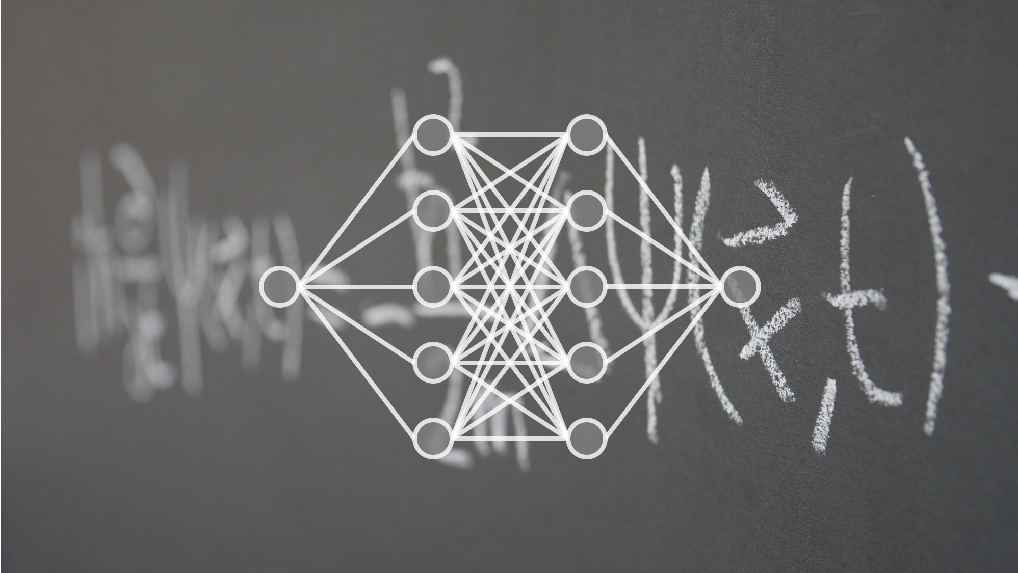
One popular way of doing this using machine learning is to use a neural network. Given the location of a data point as input (denoted x), a neural network can be used to output a prediction of its value (denoted u), as shown in the figure below:

Fig 2: schematic of a neural network

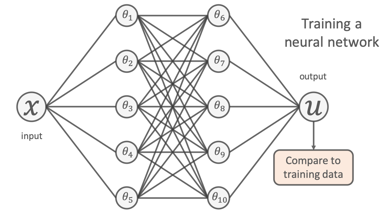
To learn a model, we try to tune the network’s free parameters (denoted by the \thetas in the figure above) so that the network’s predictions closely match the available experimental data. This is usually done by minimising the mean-squared-error between its predictions and the training points;

    \[\mathrm{min}~&\frac{1}{N} \sum^{N}_{i} (u_{\mathrm{NN}}(x_{i};\theta) - u_{\mathrm{true}}(x_i) )^2\]

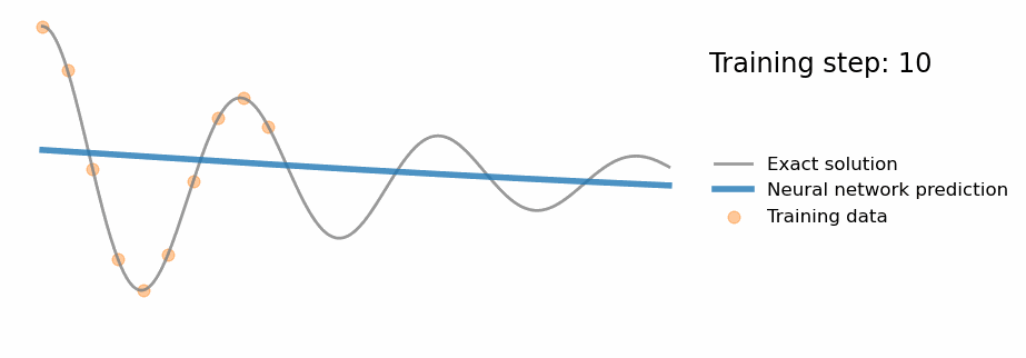
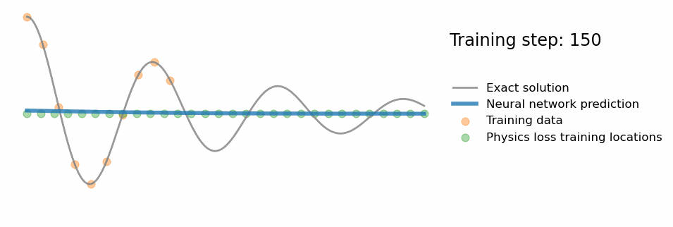
The result of training such a neural network using the experimental data above is shown in the animation.

The “naivety” of purely data-driven approaches

The problem is, using a purely data-driven approach like this can have significant downsides. Have a look at the actual values of the unknown physical process used to generate the experimental data in the animation above (grey line).

You can see that whilst the neural network accurately models the physical process within the vicinity of the experimental data, it fails to generalise away from this training data. By only relying on the data, one could argue it hasn’t truly “understood” the scientific problem.

The rise of scientific machine learning (SciML)

What if I told you that we already knew something about the physics of this process? Specifically, that the data points are actually measurements of the position of a damped harmonic oscillator:

Fig 3: a 1D damped harmonic oscillator

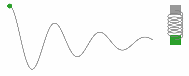
This is a classic physics problem, and we know that the underlying physics can be described by the following differential equation:

    \[m\frac{d^2u}{dx^2} + \mu \frac{du}{dx} + k u = 0\]


Where m is the mass of the oscillator, \mu is the coefficient of friction and k is the spring constant.

Given the limitations of “naive” machine learning approaches like the one above, researchers are now looking for ways to include this type of prior scientific knowledge into our machine learning workflows, in the blossoming field of scientific machine learning (SciML).

So, what is a physics-informed neural network?

One way to do this for our problem is to use a physics-informed neural network [1,2]. The idea is very simple: add the known differential equations directly into the loss function when training the neural network.

This is done by sampling a set of input training locations (\{x_{j}\}) and passing them through the network. Next gradients of the network’s output with respect to its input are computed at these locations (which are typically analytically available for most neural networks, and can be easily computed using autodifferentiation). Finally, the residual of the underlying differential equation is computed using these gradients, and added as an extra term in the loss function.

Fig 4: schematic of physics-informed neural network

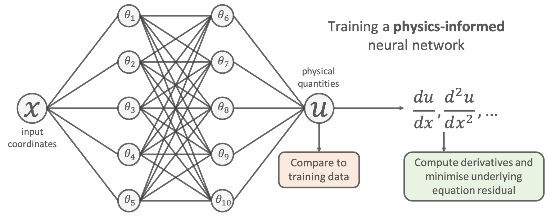
Let’s do this for the problem above. This amounts to using the following loss function to train the network:

    \begin{align*}\mathrm{min}~&\frac{1}{N} \sum^{N}_{i} (u_{\mathrm{NN}}(x_{i};\theta) - u_{\mathrm{true}}(x_i) )^2 \\+&\frac{1}{M} \sum^{M}_{j} \left( \left[ m\frac{d^2}{dx^2} + \mu \frac{d}{dx} + k \right] u_{\mathrm{NN}}(x_{j};\theta)  \right)^2\end{align}

We can see that the additional “physics loss” in the loss function tries to ensure that the solution learned by the network is consistent with the known physics.

And here’s the result when we train the physics-informed network:

Fig 5: a physics-informed neural network learning to model a harmonic oscillator

Remarks

The physics-informed neural network is able to predict the solution far away from the experimental data points, and thus performs much better than the naive network. One could argue that this network does indeed have some concept of our prior physical principles.

The naive network is performing poorly because we are “throwing away” our existing scientific knowledge; with only the data at hand, it is like trying to understand all of the data generated by a particle collider, without having been to a physics class!

Whilst we focused on a specific physics problem here, physics-informed neural networks can be easily applied to many other types of differential equations too, and are a general-purpose tool for incorporating physics into machine learning.

Conclusion

We have seen that machine learning offers a new way of carrying out scientific research, placing an emphasis on learning from data. By incorporating existing physical principles into machine learning we are able to create more powerful models that learn from data and build upon our existing scientific knowledge.

Learn more about scientific machine learning

Want to learn more about SciML? Check out my PhD thesis, and watch our ETH Zurich Deep Learning in Scientific Computing Master’s course for a great introduction to this field!

Our own work on physics-informed neural networks

We have carried out research on physics-informed neural networks! Read the following for more:

Moseley, B., Markham, A., & Nissen-Meyer, T. (2021). Finite Basis Physics-Informed Neural Networks (FBPINNs): a scalable domain decomposition approach for solving differential equations. ArXiv.

Moseley, B., Markham, A., & Nissen-Meyer, T. (2020). Solving the wave equation with physics-informed deep learning. ArXiv.

References

1. Lagaris, I. E., Likas, A., & Fotiadis, D. I. (1998). Artificial neural networks for solving ordinary and partial differential equations. IEEE Transactions on Neural Networks.

2. Raissi, M., Perdikaris, P., & Karniadakis, G. E. (2019). Physics-informed neural networks: A deep learning framework for solving forward and inverse problems involving nonlinear partial differential equations. Journal of Computational Physics.

Physics problem inspired by this blog post: https://beltoforion.de/en/harmonic_oscillator/

Seeing into permanently shadowed regions on the Moon for the first time using machine learning

As part of NASA’s Frontier Development Lab, we developed an AI algorithm which enhanced images of permanently shadowed regions on the Moon, allowing us to see into these extremely dark regions with high resolution for the first time.

Contrast-adjusted image of a permanently shadowed region (PSR) on the Moon before / after applying our AI denoising algorithm, called HORUS. For the first time, HORUS is able to see features inside the PSR such as craters and boulders down to 3-5 meters in size. Raw image credits to LROC/GSFC/ASU. Location: Kocher crater (lunar south pole).

What is a permanently shadowed region?

Read our CVPR 2021 paper here!

Whilst sunlight reaches the majority of the lunar surface, there are some places on the Moon which are covered in permanent darkness. These are called Permanently Shadowed Regions (PSRs) and they are located inside craters and other topographical depressions around the lunar poles.

At these high latitudes, and because of their shape, no direct sunlight is able to enter PSRs. An example is the Shackleton crater at the lunar south pole (shown in this post’s feature image).

Permanently shadowed regions are amongst the coldest places in the solar system, with temperatures reaching below minus 200 degrees Celsius (minus 330 Fahrenheit, or close to absolute zero). Because of these extreme conditions, PSRs have been mostly unexplored to date.

Left: Map of the Moon’s south pole, showing the location of Permanently Shadowed Regions (PSRs) (orange polygons).
Right: Lunar Reconnaissance Orbiter Narrow Angle Camera image of the Wapowski crater, which hosts a PSR. To see into the shadowed region, we first have to dramatically adjust the contrast of the image.
Image credits: LROC/GSFC/ASU/QuickMap
Contrast-adjusted image of the permanently shadowed region inside the Wapowski crater (lunar south pole) before / after applying HORUS. Raw image credits to LROC/GSFC/ASU

Searching for water

Whilst being enigmatic, PSRs are prime targets for science and exploration missions. We think they could trap water in the form of ice, which is essential for sustaining our presence on the Moon. Multiple missions are planned to study PSRs in the future; for example NASA’s VIPER rover will be driving into a PSR to search for water in 2023.

The problem is, because of their darkness, it is very difficult to see what PSRs contain. This makes it very hard to plan rover and human traverses into these regions, or to directly identify water inside of them.

Seeing in the dark

It turns out that PSRs are not completely dark. Whilst they do not receive direct sunlight, extremely small amounts of sunlight can enter PSRs by being scattered from their surroundings. Thus, we can still take photographs of PSRs, but these images usually have very poor quality.

Just like when you take a picture at night on your mobile phone, current state-of-the-art high resolution satellite images from the Lunar Reconnaissance Orbiter Narrow Angle Camera of PSRs are grainy and full of noise and this stops us making any meaningful scientific observations.

Fundamentally, this is because of the very low numbers of photons arriving at the camera. In this extreme, low-light regime, photons arrive with a large amount of randomness, producing the “graininess” in the image, and noise artefacts from the camera itself also dominate the images.

Night vision on the Moon: enhancing images of PSRs with machine learning

To overcome this problem, we used machine learning to remove the noise in these images. Our algorithm consists of two deep neural networks which target different noise components in the images. The first network removes noise generated by the camera, whilst the second network targets photon noise and any other residual noise sources in the images.

To help our algorithm learn, we developed a physical noise model of the camera and used it generate realistic training data. We also used real noise samples from calibration images, as well as 3D ray tracing of PSRs to inform our training. We named our approach HORUS, or Hyper Effective nOise Removal U-Net Software.

The HORUS noise removal software. Raw images of PSRs are very noisy (left hand side), and we used two deep neural networks to remove camera-related and photon noise from these images, producing clean images as output (right hand side).

The interactive sliders in this post show images of PSRs before and after applying HORUS. We find HORUS is able to remove large amounts of noise from these images, significantly improving their quality. Smaller craters, boulders and other geological features are revealed, making the scientific analysis and interpretation of these regions much easier.

What’s the impact?

With more analysis, our work could potentially pave the way for the direct detection of water ice or related surface features in these regions. It could also inform future rover and human scouting missions, allowing us to plan traverses into PSRs with more certainty. Our goal is to significantly impact humanity’s exploration of the Moon, helping to enable a sustainable, long term presence on the Moon and beyond.

Read the full CVPR 2021 paper here.

The team: Ben Moseley, Valentin Bickel, Ignacio Lopez-Francos, Loveneesh Rana

Our mentors: Miguel Olivares-Mendez, Dennis Wingo, Allison Zuniga

Other contributors: Nuno Subtil, Eugene D’Eon

Thanks to Leo Silverberg for designing the awesome HORUS logo.

Feature image credits: NASA’s Scientific Visualization Studio

We used AI to search for resources on the Moon

Read our NeurIPS 2019 paper here!

As part of NASA’s 2019 Frontier Development Lab, we used AI to search for resources on the surface of the Moon which could one day help humans settle there.

The Moon is a mysterious place that most of us have only seen through the lens of a telescope, but with companies like SpaceX offering commercial space flights, NASA’s new plans to put humans back on the Moon by 2024 and talk of a growing lunar economy it may start to feel much closer in the future.

Finding resources on the surface is a key part of building permanent lunar bases and sustaining our presence there.

The difficulty is that we are unsure where these resources are. Part of the problem is that the majority of the Moon is unexplored; there is a large amount of satellite data covering the surface, but without the presence of ground truth observations (i.e. humans or probes actually going there) we are not entirely confident which parts of this data correspond to resources.

Fig. 1: Optical image of the Tycho crater (approximately 120 km across). Credit: Lunar Reconnaissance Orbiter Camera

Locating metal

An important resource is metal, and one place we might expect to find it is around the Moon’s craters. We know that some of the asteroids which have impacted the Moon would have been metallic and so it is likely they left deposits in these areas.

Their temperature may be a key way to detect them. The Moon is heated by the Sun during the day and cools during the evening. Just like when you recoil from your car seatbelt in the summer because it is too hot to touch, metals are excellent at retaining their heat and we expect these craters to be hotter in the evening compared to their surroundings.

Fig. 2: Evening temperatures around the Tycho crater (left) and some examples of the temperature variation over the lunar day at different locations in and around the crater (right). Taken from the DIVINER instrument.

The DIVINER instrument aboard the Lunar Reconnaissance Orbiter has recorded the surface temperature of the Moon over 10+ years, however understanding whether a temperature anomaly relates to metal is difficult because there are many factors of variation on the lunar surface which can affect its temperature. One example is the albedo of the surface, or how reflective it is, which can affect how much heat it absorbs.

Unsupervised machine learning

We used a fully data-driven, unsupervised machine learning approach to disentangle these factors of variation in the surface temperature and uncover those which may relate to metals. We trained a variational autoencoder (VAE) to reconstruct examples of the surface temperature variation over the lunar day and then looked inside its hidden representation to understand what it found were the major factors of variation.

Fig. 3: New anomaly maps generated by our AI. Our VAE found 4 main factors of variation in the temperature variations; the plots in the bottom row show what each factor responds to in an input temperature profile and the left two columns show maps of the VAE’s latent value for each factor. We see the AI is able to disentangle the effect of albedo (latent variable 2), onset of radiation time (latent variable 1) and potentially changes in thermal conductivity relating to metal (latent variable 3).

We found that the VAE could disentangle different physical effects, such as the onset time of radiation and the albedo, allowing us to isolate and map those areas which potentially have high thermal conductivity relating to metals. Fig. 3 shows anomaly maps creating using our VAE which potentially locates metallic-like signatures over the Tycho crater.

Conclusion

Our AI-generated maps could help future mission planners and progress our vision of a fully data-driven approach to space exploration. See our final presentation below for more information!

Read the full NeurIPS 2019 workshop paper here:
https://ml4physicalsciences.github.io/2019/files/NeurIPS_ML4PS_2019_115.pdf

The team: Ben Moseley, Valentin Bickel, Jérôme Burelbach, Nicole Relatores, Daniel Angerhausen, Frank Soboczenski and Dennis Wingo

Bayesian positioning with pymc3

Today we rely on GPS for almost everything, from driving our cars to auditing our financial transactions. However when tracking animals this system is invasive because it requires the use of GPS collars. In our recent work researching elephants in Kenya, we investigated whether the vibrations elephants make through the ground could be used as an alternative way to track them.

See the full code!


In this post we will explain how we used Bayesian inference to carry out probabilistic time-difference-of-arrival positioning, using the pymc3 python library.

The problem

In this setup we have a source of vibrational waves (the elephant’s footsteps) and an array of receivers (seismometers). The receivers are synchronised in time and each measures the Time Of Arrival (TOA) of the waves at their location. In the simplest case, their TOA is given by Newton’s formula, TOA = distance between the source and receiver / speed of the waves. The goal is, given the TOA at each receiver, can we determine the location of the source?

Fig 1: The classic multilateration problem: given the time of arrival at each receiver location from a source which transmits energy waves outwards at some speed, can we determine the location of the source?

This is a classic multilateration problem and the simplest way to solve it is to draw the locus of possible source locations for each receiver and search for where they overlap (Fig. 1). However, when the time of arrival measurements are noisy and the speed of the wave is uncertain, the loci will not always overlap and this method becomes ambiguous (Fig. 2). This method also assumes we know the wave speed and the time at which the source was emitted, both of which are not always known (particularly when tracking elephants with vibrations!).

Fig 2: Noisy time of arrival measurements can result in ambiguous source positions when using the loci method.

The solution: Bayesian inference

Instead we will use some of the latest machinery for Bayesian inference in the pymc3 library to build a fully probabilistic solution to the multilateration problem. This will allow us to solve the problem without knowing the source emission time and the wave speed and quantify our uncertainty in the solution.

We represent the problem using Bayes’ theorem:

    \[ p(\mathbf{x}, v \mid \mathbf{t}) = { p(\mathbf{t} \mid \mathbf{x}, v) \, p(\mathbf{x}) \, p(v) \over p(\mathbf{t}) }\]

where the location of the source \mathbf{x}, wave speed v and observed arrival times \mathbf{t} are all random variables.

p(\mathbf{x}, v \mid \mathbf{t}) is the posterior distribution of the source location and wave speed given the arrival times and this is what we want to obtain.

The data likelihood p(\mathbf{t} \mid \mathbf{x}, v) is just the forward physics model plus observational noise and p(\mathbf{x}) and p(v) define prior distributions over the source location and wave speed which we must choose.

The difficulty in obtaining the posterior is in computing the evidence p(\mathbf{t}), which is intractable for many Bayesian inference problems.

Instead we obtain samples from the posterior using the powerful NUTS sampler in pymc3. Thankfully, pymc3 is very simple to use and the workflow only consists of two steps:

  1. Define a forward physics model
  2. Carry out inference on this model by sampling from its posterior distribution

We carry out these steps using the code below.

Step 1: define the forward model

First we define our forward model in pymc3:

import numpy as np
import pymc3 as pm
import matplotlib
import matplotlib.pyplot as plt

#stations = [array of receiver coordinates] (to be defined below)
#t_obs = [array of actual observed TDOA measurements from the receivers] (to be defined below)

with pm.Model():

    # Priors
    x = pm.Uniform("x", lower=0, upper=1000, shape=2)# prior on the source location (m)
    v = pm.Normal("v", mu=346, sigma=20)# prior on the wave speed (m/s)
    t1 = pm.Uniform("t1", lower=-2, upper=4)# prior on the time offset (s)

    # Physics
    d = pm.math.sqrt(pm.math.sum((stations - x)**2, axis=1))# distance between source and receivers
    t0 = d/v# time of arrival (TOA) of each receiver
    t = t0-t1# time difference of arrival (TDOA) from the time offset

    # Observations
    Y_obs = pm.Normal('Y_obs', mu=t, sd=0.05, observed=t_obs)# we assume Gaussian noise on the TDOA measurements

This model defines the source position and wave speed as pymc3 random variables and uses the pm.Uniform and pm.Normal classes to define their priors distributions. Newton’s equation is then used to calculate the Time-Difference-Of-Arrivals (TDOAs) at each receiver relative to some arbitrary time offset t1, using the pm.math library.

t1 is nuisance variable which would allow us to compute the source emission time if we knew its value; we must include this in our model if we are to use measurements without knowing the source emission time.

We use a normal distribution to model the observational noise and use the observed argument of the pm.Normal class to pass actual observed TDOA values from each receiver to the model.

Finally we wrap the entire model within the pm.Model(): context manager to allow pymc3 to automatically track these variables during inference.

Step 2: carry out inference

To carry out inference we generate some observations to test our model with:

# generate some test observations
N_STATIONS = 4
np.random.seed(1)
stations = np.random.randint(250,750, size=(N_STATIONS,2))# station positions (m)
x_true = np.array([500,500])# true source position (m)
v_true = 346.# speed of sound (m/s)
t1_true = 1.0# can be any constant, used to calculate TDOA values (s)
d_true = np.linalg.norm(stations-x_true, axis=1)
t0_true = d_true/v_true# true time of flight values
t_obs = t0_true-t1_true# true time difference of arrival values
np.random.seed(1)
t_obs = t_obs+0.05*np.random.randn(*t_obs.shape)# noisy observations
print("t_obs (s):", t_obs)

# t_obs and stations are passed to the pymc3 model above

# plot them
plt.figure(figsize=(5,5))
plt.scatter(stations[:,0], stations[:,1], marker="^", s=80, label="Receivers")
plt.scatter(x_true[0], x_true[1], s=40, label="True source position")
plt.legend(loc=2)
plt.xlim(250, 750)
plt.ylim(250, 750)
plt.xlabel("x (m)")
plt.ylabel("y (m)")

t_obs (s): [-0.30165118 -0.36521993 -0.61286123 -0.68923435]

and then sample from the posterior of our model by using:

# Sample posterior
trace = pm.sample(draws=2000,
                  tune=2000,
                  chains=4,
                  target_accept=0.95,
                  init='jitter+adapt_diag')

pymc3 auto-assigns the NUTS sampler and draws 2000 samples from the posterior, which are stored in the trace object. All we need to do is plot these samples to obtain an estimate of the location with its associated uncertainty, and we are done!

# get means and standard deviations of posterior samples
summary = pm.summary(trace)
mu = np.array(summary["mean"])
sd = np.array(summary["sd"])

# plot
plt.figure(figsize=(5,5))
plt.scatter(stations[:,0], stations[:,1], marker="^", s=80, label="Receivers")
plt.scatter(x_true[0], x_true[1], s=40, label="True source position")
ell = matplotlib.patches.Ellipse(xy=(mu[1], mu[2]),
          width=4*sd[1], height=4*sd[2],
          angle=0., color='black', label="Posterior (2\sigma)", lw=1.5)
ell.set_facecolor('none')
plt.gca().add_patch(ell)
plt.legend(loc=2)
plt.xlim(250, 750)
plt.ylim(250, 750)
plt.xlabel("x (m)")
plt.ylabel("y (m)")

Checking the convergence of the sampler

pymc3 includes some useful tools for checking that the sampler has converged correctly. One thing we can do is to call the pm.traceplot(trace) function to plot the samples and posterior distributions of each of the variables:

Using the velocity prior as a regulariser


A neat thing about using a Bayesian framework is that the wave speed prior p(v) regularises our solution. Note that we would typically need 4 receivers to solve for the source coordinates, TOAs of the receivers and the wave speed. However, with a strong enough wave speed prior, we can get away with only 3 receivers. By switching N_STATIONS = 3 in the code above, we obtain:

Conclusion

We have built a probabilistic time-difference-of-arrival positioning method using the pymc3 library. This allows us to solve the multilateration problem without knowing the source emission time and the wave speed and quantify our uncertainty in the solution.

See the full code here: https://github.com/benmoseley/bayesian-time-difference-of-arrival-positioning

Can we track elephants using the vibrations they make through the ground?

In February this year I joined a research trip in Kenya and helped to investigate whether it is possible to track elephants using the vibrations they make through the ground.

Many elephants suffer from poaching, habitat destruction and conflicts with local people and being able to track them more effectively would aid conservation efforts.

Current techniques, such as positioning based on satellite imagery, camera traps or acoustic sensing, either lack temporal resolution, are expensive, or are limited to small areas. One solution which may address these challenges is to track elephants using the vibrations they make.

Elephants make vibrations through the ground as they walk

Elephants have many different types of behaviour which generate ground vibrations, including running, playing, bathing and walking. They also make low-frequency vocalisations known as “rumbling”, thought to be a means of communication between elephants, which propagate vibrations into the ground.

A key benefit of using these vibrations is that we think they can travel long distances, potentially allowing us to track the elephants over large areas and at low cost.

We listen for vibrations in the ground using seismometers, which are buried in the ground and are therefore non-invasive. These vibrations are noisy and hard to interpret; we are investigating the use of AI to help us accurately identify and locate the signals made by elephants.

We record the vibrations the elephants make using seismometers buried in the ground

Once we are able to accurately detect elephants, we will use Bayesian positioning to accurately locate them (see my other post on this).

See more info here: https://www.eng.ox.ac.uk/news/track-elephants-vibrations-footsteps/

Hello world!

Brand new website launched!

I am excited to launch the website (it’s my first forage into website development so bear with me..), watch out for posts on AI and machine learning soon!