Machine learning has become increasingly popular across science, but do these algorithms actually “understand” the scientific problems they are trying to solve? In this article we explain physics-informed neural networks, which are a powerful way of incorporating physical principles into machine learning.
A machine learning revolution in science
Machine learning has caused a fundamental shift in the scientific method. Traditionally, scientific research has revolved around theory and experiment: one hand-designs a well-defined theory and then continuously refines it using experimental data and analyses it to make new predictions.
But today, with rapid advances in the field of machine learning and dramatically increasing amounts of scientific data, data-driven approaches have become increasingly popular. Here an existing theory is not required, and instead a machine learning algorithm can be used to analyse a scientific problem using data alone.
Learning to model experimental data
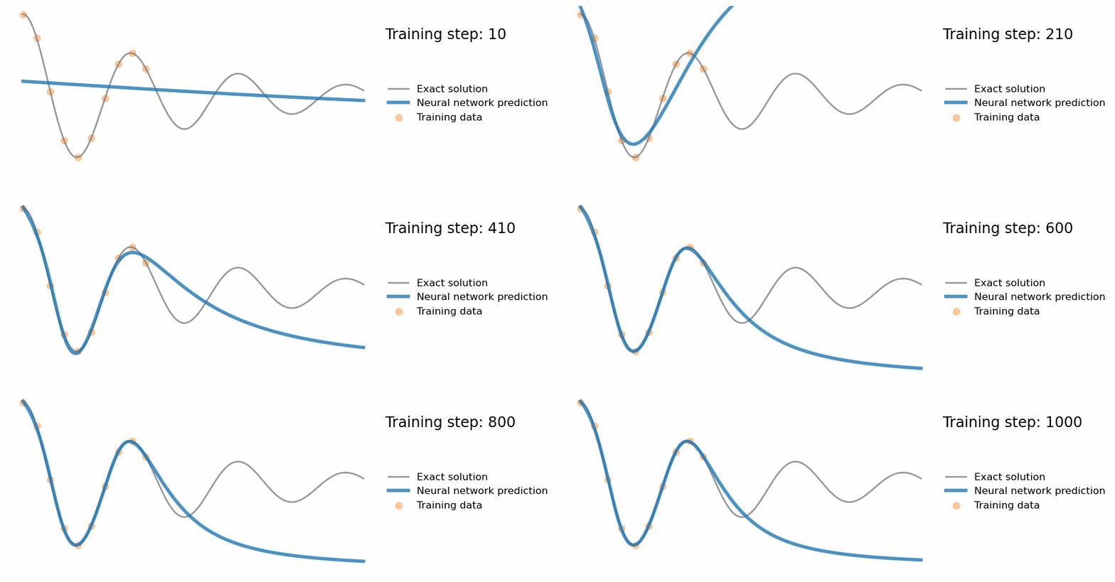
Let’s look at one way machine learning can be used for scientific research. Imagine we are given some experimental data points that come from some unknown physical phenomenon, e.g. the orange points in the animation below.
A common scientific task is to find a model which is able to accurately predict new experimental measurements given this data.
One popular way of doing this using machine learning is to use a neural network. Given the location of a data point as input (denoted ![]() ), a neural network can be used to output a prediction of its value (denoted
), a neural network can be used to output a prediction of its value (denoted ![]() ), as shown in the figure below:
), as shown in the figure below:
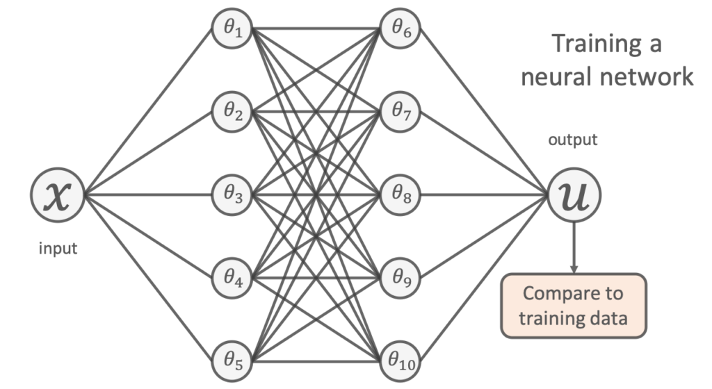
To learn a model, we try to tune the network’s free parameters (denoted by the ![]() s in the figure above) so that the network’s predictions closely match the available experimental data. This is usually done by minimising the mean-squared-error between its predictions and the training points;
s in the figure above) so that the network’s predictions closely match the available experimental data. This is usually done by minimising the mean-squared-error between its predictions and the training points;
![Rendered by QuickLaTeX.com \[\mathrm{min}~&\frac{1}{N} \sum^{N}_{i} (u_{\mathrm{NN}}(x_{i};\theta) - u_{\mathrm{true}}(x_i) )^2\]](https://benmoseley.blog/wp-content/ql-cache/quicklatex.com-6d5ab22a997dad99353f6f83b9e5f092_l3.png)
The result of training such a neural network using the experimental data above is shown in the animation.
The “naivety” of purely data-driven approaches
The problem is, using a purely data-driven approach like this can have significant downsides. Have a look at the actual values of the unknown physical process used to generate the experimental data in the animation above (grey line).
You can see that whilst the neural network accurately models the physical process within the vicinity of the experimental data, it fails to generalise away from this training data. By only relying on the data, one could argue it hasn’t truly “understood” the scientific problem.
The rise of scientific machine learning (SciML)
What if I told you that we already knew something about the physics of this process? Specifically, that the data points are actually measurements of the position of a damped harmonic oscillator:
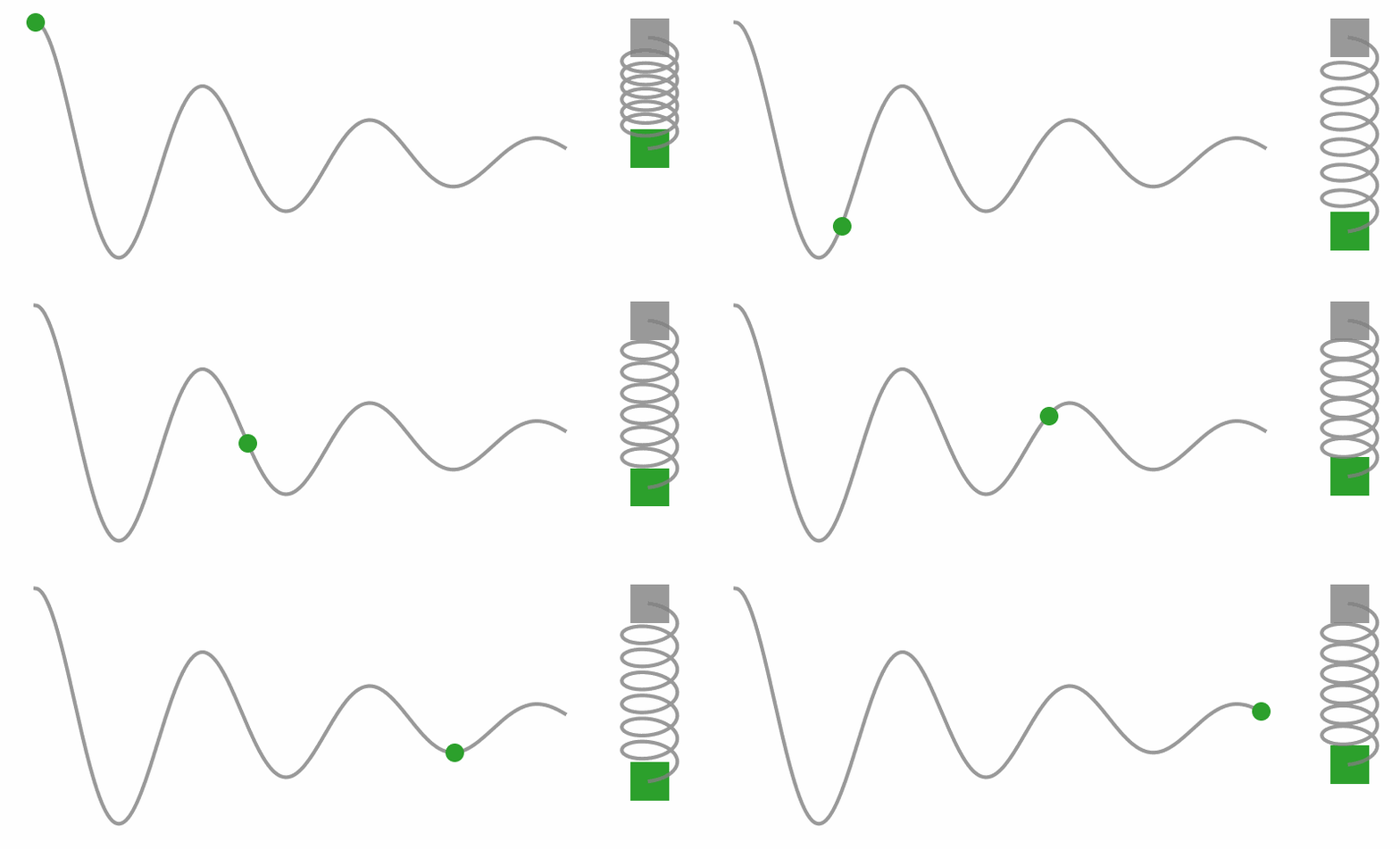
This is a classic physics problem, and we know that the underlying physics can be described by the following differential equation:
![]()
Where
Given the limitations of “naive” machine learning approaches like the one above, researchers are now looking for ways to include this type of prior scientific knowledge into our machine learning workflows, in the blossoming field of scientific machine learning (SciML).
So, what is a physics-informed neural network?
One way to do this for our problem is to use a physics-informed neural network [1,2]. The idea is very simple: add the known differential equations directly into the loss function when training the neural network.
This is done by sampling a set of input training locations (![]() ) and passing them through the network. Next gradients of the network’s output with respect to its input are computed at these locations (which are typically analytically available for most neural networks, and can be easily computed using autodifferentiation). Finally, the residual of the underlying differential equation is computed using these gradients, and added as an extra term in the loss function.
) and passing them through the network. Next gradients of the network’s output with respect to its input are computed at these locations (which are typically analytically available for most neural networks, and can be easily computed using autodifferentiation). Finally, the residual of the underlying differential equation is computed using these gradients, and added as an extra term in the loss function.
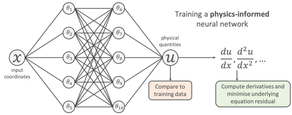
Let’s do this for the problem above. This amounts to using the following loss function to train the network:
![Rendered by QuickLaTeX.com \begin{align*}\mathrm{min}~&\frac{1}{N} \sum^{N}_{i} (u_{\mathrm{NN}}(x_{i};\theta) - u_{\mathrm{true}}(x_i) )^2 \\+&\frac{1}{M} \sum^{M}_{j} \left( \left[ m\frac{d^2}{dx^2} + \mu \frac{d}{dx} + k \right] u_{\mathrm{NN}}(x_{j};\theta) \right)^2\end{align}](https://benmoseley.blog/wp-content/ql-cache/quicklatex.com-e464074c612008eafebb82a1faa49bde_l3.png)
We can see that the additional “physics loss” in the loss function tries to ensure that the solution learned by the network is consistent with the known physics.
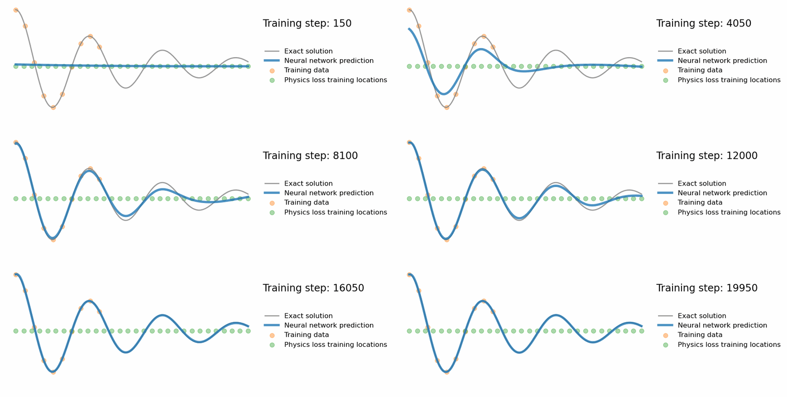
And here’s the result when we train the physics-informed network:
Remarks
The physics-informed neural network is able to predict the solution far away from the experimental data points, and thus performs much better than the naive network. One could argue that this network does indeed have some concept of our prior physical principles.
The naive network is performing poorly because we are “throwing away” our existing scientific knowledge; with only the data at hand, it is like trying to understand all of the data generated by a particle collider, without having been to a physics class!
Whilst we focused on a specific physics problem here, physics-informed neural networks can be easily applied to many other types of differential equations too, and are a general-purpose tool for incorporating physics into machine learning.
Conclusion
We have seen that machine learning offers a new way of carrying out scientific research, placing an emphasis on learning from data. By incorporating existing physical principles into machine learning we are able to create more powerful models that learn from data and build upon our existing scientific knowledge.
Learn more about scientific machine learning
Want to learn more about SciML? Check out my PhD thesis, and watch our ETH Zurich Deep Learning in Scientific Computing Master’s course for a great introduction to this field!
Our own work on physics-informed neural networks
We have carried out research on physics-informed neural networks! Read the following for more:
Moseley, B., Markham, A., & Nissen-Meyer, T. (2023). Finite Basis Physics-Informed Neural Networks (FBPINNs): a scalable domain decomposition approach for solving differential equations. Advances in Computational Mathematics.
Moseley, B., Markham, A., & Nissen-Meyer, T. (2020). Solving the wave equation with physics-informed deep learning. ArXiv.
References
1. Lagaris, I. E., Likas, A., & Fotiadis, D. I. (1998). Artificial neural networks for solving ordinary and partial differential equations. IEEE Transactions on Neural Networks.
2. Raissi, M., Perdikaris, P., & Karniadakis, G. E. (2019). Physics-informed neural networks: A deep learning framework for solving forward and inverse problems involving nonlinear partial differential equations. Journal of Computational Physics.
Physics problem inspired by this blog post: https://beltoforion.de/en/harmonic_oscillator/
