Bayesian positioning with pymc3

Today we rely on GPS for almost everything, from driving our cars to auditing our financial transactions. However when tracking animals this system is invasive because it requires the use of GPS collars. In our recent work researching elephants in Kenya, we investigated whether the vibrations elephants make through the ground could be used as an alternative way to track them.

In this post we will explain how we used Bayesian inference to carry out probabilistic time-difference-of-arrival positioning, using the pymc3 python library.

The problem

In this setup we have a source of vibrational waves (the elephant’s footsteps) and an array of receivers (seismometers). The receivers are synchronised in time and each measures the Time Of Arrival (TOA) of the waves at their location. In the simplest case, their TOA is given by Newton’s formula, TOA = distance between the source and receiver / speed of the waves. The goal is, given the TOA at each receiver, can we determine the location of the source?

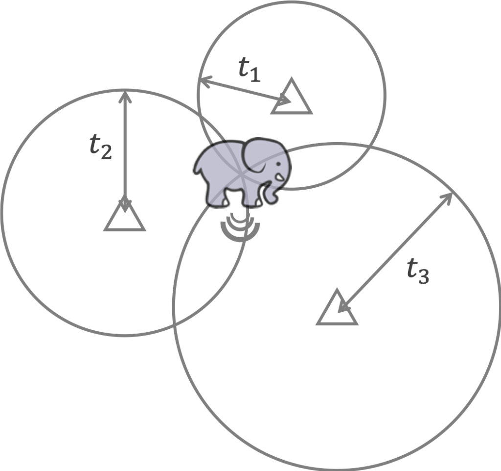
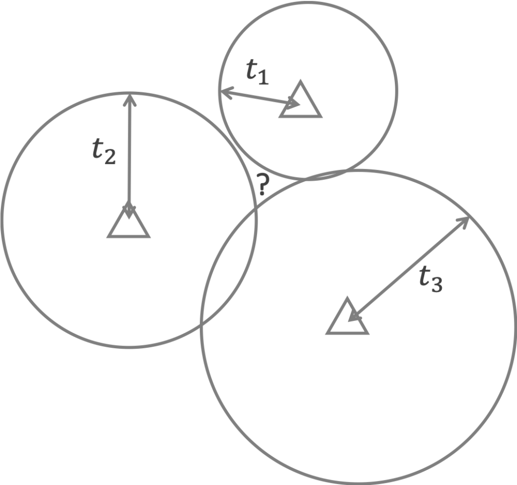
This is a classic multilateration problem and the simplest way to solve it is to draw the locus of possible source locations for each receiver and search for where they overlap (Fig. 1). However, when the time of arrival measurements are noisy and the speed of the wave is uncertain, the loci will not always overlap and this method becomes ambiguous (Fig. 2). This method also assumes we know the wave speed and the time at which the source was emitted, both of which are not always known (particularly when tracking elephants with vibrations!).

The solution: Bayesian inference

Instead we will use some of the latest machinery for Bayesian inference in the pymc3 library to build a fully probabilistic solution to the multilateration problem. This will allow us to solve the problem without knowing the source emission time and the wave speed and quantify our uncertainty in the solution.

We represent the problem using Bayes’ theorem:

1. Define a forward physics model
2. Carry out inference on this model by sampling from its posterior distribution

We carry out these steps using the code below.

Step 1: define the forward model

First we define our forward model in pymc3:

import numpy as np
import pymc3 as pm
import matplotlib
import matplotlib.pyplot as plt

#stations = [array of receiver coordinates] (to be defined below)
#t_obs = [array of actual observed TDOA measurements from the receivers] (to be defined below)

with pm.Model():

    # Priors
    x = pm.Uniform("x", lower=0, upper=1000, shape=2)# prior on the source location (m)
    v = pm.Normal("v", mu=346, sigma=20)# prior on the wave speed (m/s)
    t1 = pm.Uniform("t1", lower=-2, upper=4)# prior on the time offset (s)

    # Physics
    d = pm.math.sqrt(pm.math.sum((stations - x)**2, axis=1))# distance between source and receivers
    t0 = d/v# time of arrival (TOA) of each receiver
    t = t0-t1# time difference of arrival (TDOA) from the time offset

    # Observations
    Y_obs = pm.Normal('Y_obs', mu=t, sd=0.05, observed=t_obs)# we assume Gaussian noise on the TDOA measurements

This model defines the source position and wave speed as pymc3 random variables and uses the pm.Uniform and pm.Normal classes to define their priors distributions. Newton’s equation is then used to calculate the Time-Difference-Of-Arrivals (TDOAs) at each receiver relative to some arbitrary time offset t1, using the pm.math library.

t1 is nuisance variable which would allow us to compute the source emission time if we knew its value; we must include this in our model if we are to use measurements without knowing the source emission time.

We use a normal distribution to model the observational noise and use the observed argument of the pm.Normal class to pass actual observed TDOA values from each receiver to the model.

Finally we wrap the entire model within the pm.Model(): context manager to allow pymc3 to automatically track these variables during inference.

Step 2: carry out inference

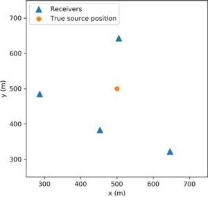
To carry out inference we generate some observations to test our model with:

# generate some test observations
N_STATIONS = 4
np.random.seed(1)
stations = np.random.randint(250,750, size=(N_STATIONS,2))# station positions (m)
x_true = np.array([500,500])# true source position (m)
v_true = 346.# speed of sound (m/s)
t1_true = 1.0# can be any constant, used to calculate TDOA values (s)
d_true = np.linalg.norm(stations-x_true, axis=1)
t0_true = d_true/v_true# true time of flight values
t_obs = t0_true-t1_true# true time difference of arrival values
np.random.seed(1)
t_obs = t_obs+0.05*np.random.randn(*t_obs.shape)# noisy observations
print("t_obs (s):", t_obs)

# t_obs and stations are passed to the pymc3 model above

# plot them
plt.figure(figsize=(5,5))
plt.scatter(stations[:,0], stations[:,1], marker="^", s=80, label="Receivers")
plt.scatter(x_true[0], x_true[1], s=40, label="True source position")
plt.legend(loc=2)
plt.xlim(250, 750)
plt.ylim(250, 750)
plt.xlabel("x (m)")
plt.ylabel("y (m)")

t_obs (s): [-0.30165118 -0.36521993 -0.61286123 -0.68923435]

and then sample from the posterior of our model by using:

# Sample posterior
trace = pm.sample(draws=2000,
                  tune=2000,
                  chains=4,
                  target_accept=0.95,
                  init='jitter+adapt_diag')

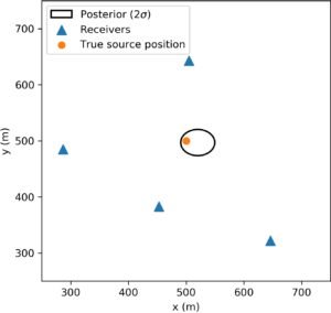
pymc3 auto-assigns the NUTS sampler and draws 2000 samples from the posterior, which are stored in the trace object. All we need to do is plot these samples to obtain an estimate of the location with its associated uncertainty, and we are done!

# get means and standard deviations of posterior samples
summary = pm.summary(trace)
mu = np.array(summary["mean"])
sd = np.array(summary["sd"])

# plot
plt.figure(figsize=(5,5))
plt.scatter(stations[:,0], stations[:,1], marker="^", s=80, label="Receivers")
plt.scatter(x_true[0], x_true[1], s=40, label="True source position")
ell = matplotlib.patches.Ellipse(xy=(mu[1], mu[2]),
          width=4*sd[1], height=4*sd[2],
          angle=0., color='black', label="Posterior ()", lw=1.5)
ell.set_facecolor('none')
plt.gca().add_patch(ell)
plt.legend(loc=2)
plt.xlim(250, 750)
plt.ylim(250, 750)
plt.xlabel("x (m)")
plt.ylabel("y (m)")

Checking the convergence of the sampler

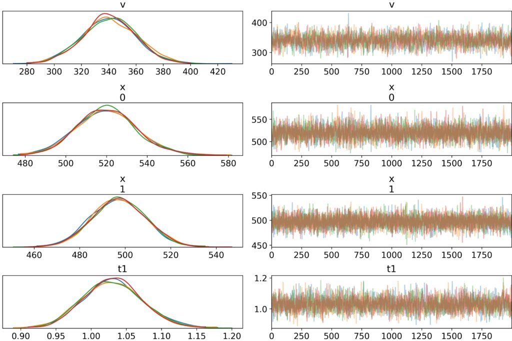
pymc3 includes some useful tools for checking that the sampler has converged correctly. One thing we can do is to call the pm.traceplot(trace) function to plot the samples and posterior distributions of each of the variables:

Using the velocity prior as a regulariser

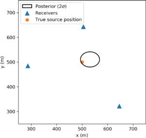
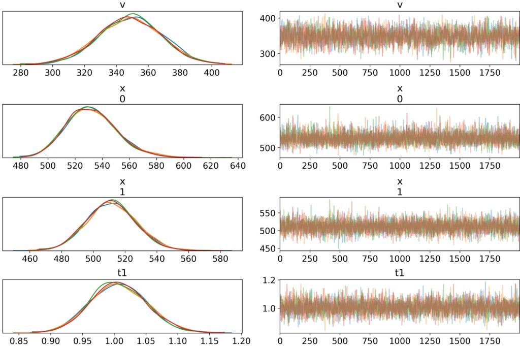
A neat thing about using a Bayesian framework is that the wave speed prior regularises our solution. Note that we would typically need 4 receivers to solve for the source coordinates, TOAs of the receivers and the wave speed. However, with a strong enough wave speed prior, we can get away with only 3 receivers. By switching N_STATIONS = 3 in the code above, we obtain:

Conclusion

We have built a probabilistic time-difference-of-arrival positioning method using the pymc3 library. This allows us to solve the multilateration problem without knowing the source emission time and the wave speed and quantify our uncertainty in the solution.

See the full code here: https://github.com/benmoseley/bayesian-time-difference-of-arrival-positioning